Dynamic Assignment in VISSIM
Dynamic Assignment in VISSIM – Some (Updated) Thoughts & Suggestions
The use of dynamic assignment in VISSIM models can be considered a ‘dark art’, with very little content online which demonstrates how to go about this process and what the key elements are to look out for.
As a result, we wanted to share our thoughts and current methodology to a wider audience. We are aware that there is no ‘one best solution’ to undertaking dynamic assignment, but hope this helps to generate further debate and/ or improvement and provide some help to those who are looking for a starting point with dynamic assignment.
A bit of background…
Before the introduction of Equilibrium Assignment in VISSIM 9, VISSIM models developed with dynamic assignment routing were generally configured to use the Kirchhoff (Stochastic assignment) option, with user specified ‘path pre-selection’ parameters and an MSA (Method of Successive Averages) option for Cost Running (see Figure 1).

Figure 1 - Dynamic Assignment Parameters - VISSIM 8
However, in VISSIM 9, we now have the introduction of Equilibrium Assignment, which in our experience has muddied the waters a little bit. We understand the premise of it (balancing the traffic flows between paths to favour the less congested routes) but having tried to use it on a previous project, we could not develop a suitable path file for meeting TAG calibration and validation criteria.
This may have been down to us not fully grasping the concept and choosing appropriate supporting path search criteria, but in the end, we chose to use the Stochastic Assignment in order to continue getting the results we wanted.
Step forward to now…
We have been working on a model of a small town, with route choice required to be modelled to asses the impact of proposed relief road options in a future year. We followed our normal Stochastic Assignment routing methodology and together with link/ connector surcharges, produced a calibrated and validated model. However, when it came to assessing the impact of the future year relief roads, the added surcharges were causing problems, with the new path files not producing routes as expected.
We were then faced with two options – 1) remove the surcharges and proceed with Stochastic Assignment (which then becomes a grey area as the model is calibrated and validated with these surcharges in place), or 2) explore the use of Equilibrium Assignment to see if this produced more sensible paths (which also meant removing the surcharges and if successful, re-checking the base model calibration/ validation levels with this assignment option in place).
We decided to proceed with option 2) on the basis that, if we could get a calibrated and validated base model without needing surcharges, then it would make the future year testing a more straight-forward process.
Stage 1 – Equilibrium Assignment – Path File Running
We set up the model to run for an initial path file, with the configuration set out in Figure 2.
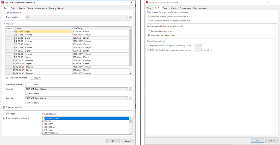

Figure 2 - Equilibrium Assignment Parameters - Path File Running - VISSIM 9
The key points to note on the path file running:
- We are not storing for Costs and not penalising routes with excessive cost – this produced a better initial path to take forward for Cost running.
- We had to undertake a couple of iterations to ensure that the ‘Avoid Long Detours’ factor was suitable for our network. A factor too high produced unrealistic paths, whilst a figure too low didn’t find enough suitable paths.
- The models were run using a reduced demand to start with and then increased through multiple runs of different seeds.
Stage 2 – Equilibrium Assignment – Cost File Running
We set up the model to run for an initial cost file, with the configuration set out in Figure 3.

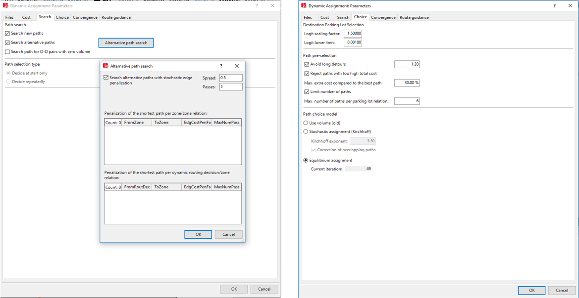
Figure 3 - Equilibrium Assignment Parameters - Cost File Running - VISSIM 9
The key points to note on the cost file running:
- ‘Store Costs’ and ‘Reject paths with too high cost…’ options are now selected as we now wanted the cost and path file to take into account the costs on routes.
- We continued to run the cost file with ‘Search New Paths’ As we ran creating archive files, we found that even with this ticked, the size of the path file eventually stabilised through multiple seed runs.
As with the path file, the models were run using a reduced demand to start with and then increased through multiple runs of different seeds. This was done over a large number of seed runs to ‘bed in’ the cost file and allow variance between the runs to be accounted for over a larger sample size. We also chose to collect the ‘archive files’ and direct ‘convergence’ outputs from the model, so that we could track the file size of the *BEW file and interrogate the *CVA files to understand how stable the cost file was.
Stage 3 – Equilibrium Assignment – Convergence Running
We set up the model to run for convergence, with the configuration set out in Figure 4.

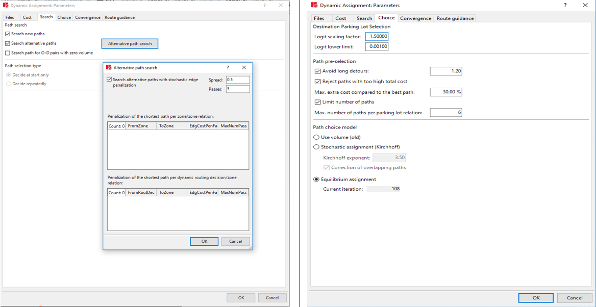
Figure 4 - Equilibrium Assignment Parameters - Convergence Running - VISSIM 9
The key points to note on the convergence running:
- The ‘scale total volume…’ is unticked so that 100% of the traffic is run each time.
- We continued to have the ‘Search new paths’ option ticked. As our model contained decimal numbers in the O-D matrices, having this ticked removed previous errors of missing vehicles when running for multiple seeds. We also found that, as with the cost file run, by reviewing the archived files, the path file was not changing from run to run and not having a significant effect on the convergence of the model. It should be noted that, if the matrices are made up of whole numbers (i.e. no decimal places), then ‘Search new paths’ should be unticked.
- The model was run multiple times whilst exporting both the network performance and direct CVA outputs, on the same seed to check convergence against TAG
Stage 4 – Equilibrium Assignment – Results Running
We set up the model to run for results, with the configuration set out in Figure 5.
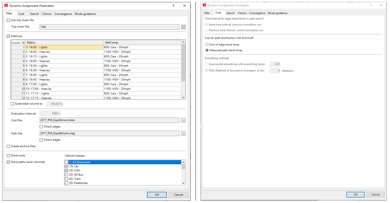

Figure 5 - Equilibrium Assignment Parameters - Results Running - VISSIM 9
The key points to note on the results running:
- The option to ‘Store Costs’ is now unticked as we want to preserve the cost file chosen as most suitable and stable from the Convergence running analysis.
- We continued to have ‘Search new paths’ options ticked due to the O-D matrices having decimal places. This removes the errors of vehicles not being able to leave the parking lot, without affecting the path file. It should be noted that in ‘normal’ circumstances, the O-D matrices will be made up of whole numbers (i.e. no decimal places), meaning ‘Search new paths’ does not need to be ticked. This preserves the path file chosen from the Convergence running analysis.
- The model was run multiple times on different seeds to obtain a suitable average for results reporting.
The Outcomes…
Convergence
Following the process detailed above, the convergence results obtained are shown in Figure 6.

Figure 6 - Equilibrium Assignment Parameters - Convergence Results - VISSIM 9
It can be seen that majority of the TAG convergence criteria was met, with the Volume Difference and Travel Time on Edges problematic (in our experience, notoriously so on many models) in the AM peak.
Calibration & Validation
In terms of the calibration and validation results, the flow and journey time results were improved over the Stochastic Assignment method.
Future Year Testing
Taking this Equilibrium Assignment methodology forward into the future year testing, the traffic assignment as a result of proposed relief roads appeared much more realistic and produced results which were more in line with what was to be expected. The lack of surcharges to inform route choice certainly seemed to help traffic reassign more freely around the network.
Final Thoughts…
The use of Equilibrium Assignment for Dynamic Assignment routing certainly seems to have its advantages, particularly in models with route choice. That being said, there has been some lessons learned in terms of how important it is to get the path pre-selection parameters correct to start with and the need to have ‘store costs’ and ‘search new paths’ checked throughout the whole process.
As mentioned at the start, this is certainly not the only approach to undertaking dynamic assignment and may still require further refinements. However, with recent queries on the subject, we felt it was worthwhile producing something to demonstrate how Equilibrium Assignment has been successful and what methodology and parameters were used/checked to achieve our goal.
We hope this helps and please feedback with any comments.
Extended Thoughts…What about Stochastic Assignment?
Whilst this post has specifically focused on Equilibrium Assignment, what about if you want to use Stochastic Assignment as your choice of path model?
Well, the steps already identified can still be followed and the key differences in the dynamic assignment set-up are shown in Figure 7.
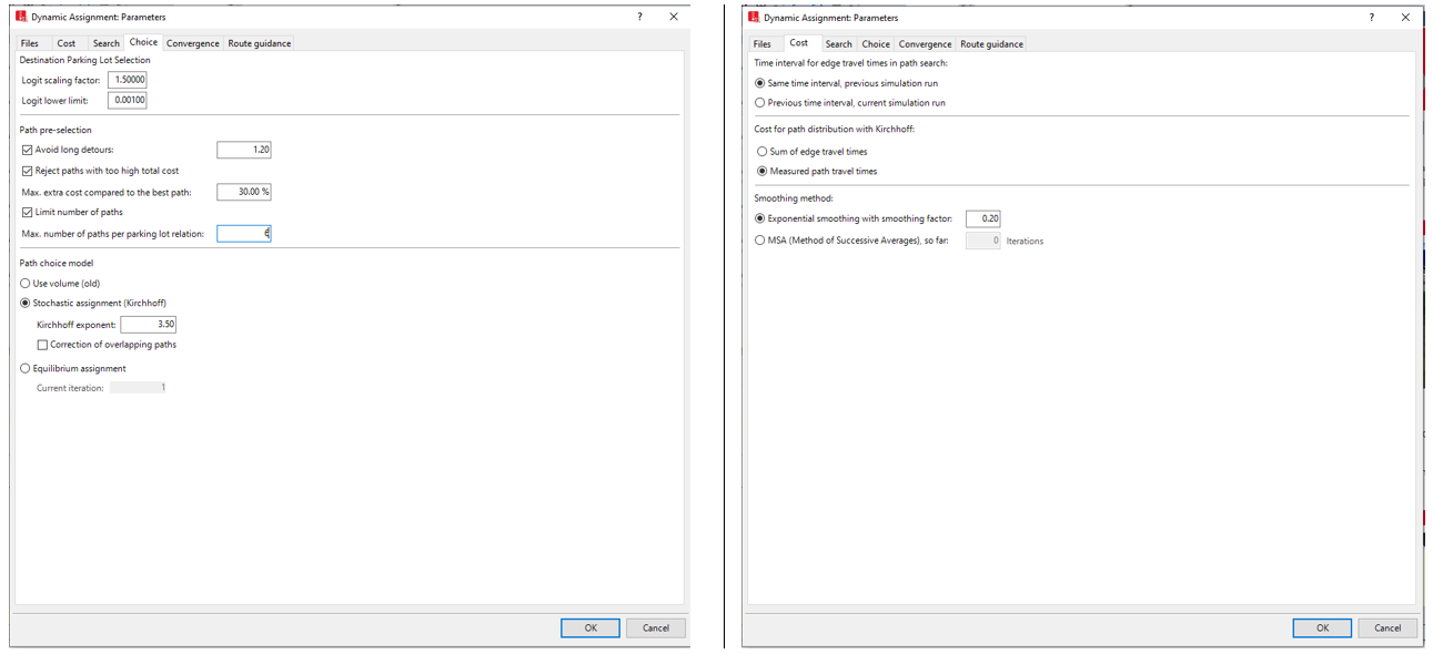
Figure 7 - Stochastic Assignment Parameters
The key differences to note are:
- Within the ‘Choice’ tab, the Stochastic assignment (Kirchhoff) has been chosen instead of Equilibrium Assignment
- Within the ‘Cost’ tab, the following change are made:
- The cost for path distribution is amended to ‘Measured path travel times’
- The smoothing method is set to ‘Exponential smoothing’ with a default value of 0.20.
The use of ‘Measured path travel times’ over ‘Sum of edge travel times’ is based on guidance in the VISSIM manual. This states that for links with multiple lanes and for congested networks, the measured path travel times produces more accurate results.
For the smoothing method, the ‘Method of Successive Averages (MSA)’ can be chosen. If using this method, it is important to update the number of iterations after each stage of the dynamic assignment process. For example, if the model is run 20 times for paths, 20 times for costs and then 100 times for convergence, the following MSA values should be entered – 20, 40 and 140 iterations.
Hope this helps and any questions or comments, do get in touch!